Practical Evolutionary Algorithms

A practical book on Evolutionary Algorithms that teaches you the concepts and how they’re implemented in practice.

Get the book
Pareto-Front Visualisation with PlotAPI

Preamble

from plotapi import ParetoFront

Introduction

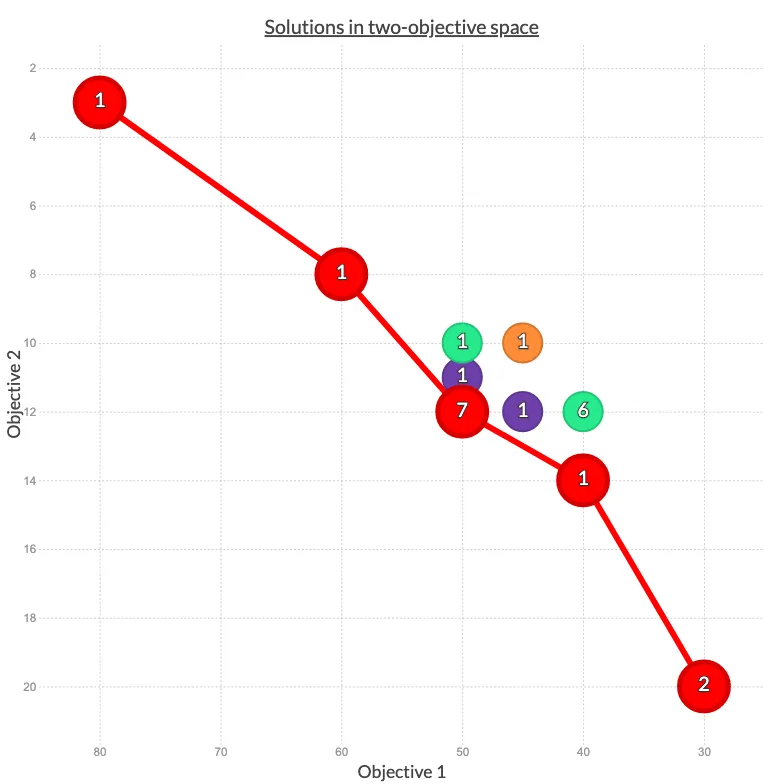
Dominance relations can be clearly visualised when working in a two-objective space. Such visualisations can be useful for:

  • Monitoring performance throughout the optimisation process.
  • Understanding and exploring spatial relationships.
  • Presentation to a decision maker.
  • Progressive and interactive preference articulation throughout the optimisation process1.

We'll use the PlotAPI package which is available for Python, Rust, JavaScript, Ruby, Julia, and any language that supports HTTP requests. PlotAPI has a specialised multi-objective visualisation type for displaying Pareto and Non-Dominated fronts, named ParetoFront.

Solutions in Objective Space

Let's do this with some arbitrary solutions.

solutions = [
    {"order": 0, "objv_1": 40, "objv_2": 12},
    {"order": 0, "objv_1": 40, "objv_2": 12},
    {"order": 0, "objv_1": 40, "objv_2": 12},
    {"order": 0, "objv_1": 40, "objv_2": 12},
    {"order": 0, "objv_1": 40, "objv_2": 12},
    {"order": 0, "objv_1": 40, "objv_2": 14},
    {"order": 0, "objv_1": 40, "objv_2": 12},
    {"order": 0, "objv_1": 45, "objv_2": 12},
    {"order": 0, "objv_1": 45, "objv_2": 10},
    {"order": 0, "objv_1": 50, "objv_2": 12},
    {"order": 0, "objv_1": 50, "objv_2": 11},
    {"order": 0, "objv_1": 50, "objv_2": 10},
    {"order": 0, "objv_1": 50, "objv_2": 12},
    {"order": 0, "objv_1": 50, "objv_2": 12},
    {"order": 0, "objv_1": 50, "objv_2": 12},
    {"order": 0, "objv_1": 50, "objv_2": 12},
    {"order": 0, "objv_1": 50, "objv_2": 12},
    {"order": 0, "objv_1": 50, "objv_2": 12},
    {"order": 0, "objv_1": 60, "objv_2": 8},
    {"order": 0, "objv_1": 80, "objv_2": 3},
    {"order": 0, "objv_1": 30, "objv_2": 20},
    {"order": 0, "objv_1": 30, "objv_2": 20},
    {"order": 0, "objv_1": 10, "objv_2": 20},
]

Here we can see our population defined as a list of dictionary items. Each dictionary includes:

  • order which determines with time period this item belongs to. This should be numerical, but can be formatted e.g. as dates.
  • objv_1 the first objective value, e.g. "speed".
  • objv_2 the second objective value, e.g. "cost".

Visualisation

A Simple and Static Visualisation

Let's demonstrate solutions plotted in two-objective space.

Here, we've disabled most of PlotAPI's features to replicate the visualisation from the Sections on Pareto Optimality and Dominance Relations and Non-Dominated Sorting.

ParetoFront(
    solutions,
    popup_enabled=False,
    show_order=False,
    zoomed=False,
    current_order_highlight=False,
    show_pareto_front=False,
    transition_delay=0,
    transition_duration=0,
    label_font_size=0,
    event_font_size=0,
    x_label="Objective 1",
    y_label="Objective 2",
    optimisations=["max", "max"],
).show()
PlotAPI - ParetoFront Diagram

An Interactive Visualisation

Now let's leverage more of PlotAPI's features to visualise the same set.

Hovering over a solution will display a pop with more information, and highlight solutions of the same non-dominated rank. Clicking on the visualisation will switch the view scope between focussing on Pareto Front solutions and displaying all solutions.

ParetoFront(
    solutions,
    show_order=False,
    current_order_highlight=False,
    x_label="Objective 1",
    y_label="Objective 2",
    optimisations=["max", "max"],
    title="Solutions in two-objective space"
).show()

An animated visualisation

Let's demonstrate the same visualisation applied to solutions over time.

solutions = [
    {'order': 20200101, 'objv_1': 40, 'objv_2': 12},   
    {'order': 20200101, 'objv_1': 40, 'objv_2': 12},   
    {'order': 20200101, 'objv_1': 40, 'objv_2': 12},   

    {'order': 20200104, 'objv_1': 40, 'objv_2': 12},   
    {'order': 20200104, 'objv_1': 40, 'objv_2': 12},   
    {'order': 20200104, 'objv_1': 40, 'objv_2': 14},   

    {'order': 20200109, 'objv_1': 40, 'objv_2': 12},   
    {'order': 20200109, 'objv_1': 45, 'objv_2': 12},   
    {'order': 20200109, 'objv_1': 45, 'objv_2': 10},   

    {'order': 20200112, 'objv_1': 50, 'objv_2': 12},   
    {'order': 20200112, 'objv_1': 50, 'objv_2': 11},   
    {'order': 20200112, 'objv_1': 50, 'objv_2': 10},   

    {'order': 20200115, 'objv_1': 50, 'objv_2': 12},   
    {'order': 20200115, 'objv_1': 50, 'objv_2': 12},   
    {'order': 20200115, 'objv_1': 50, 'objv_2': 12},   

    {'order': 20200115, 'objv_1': 50, 'objv_2': 12},   
    {'order': 20200115, 'objv_1': 50, 'objv_2': 12},   
    {'order': 20200115, 'objv_1': 50, 'objv_2': 12},   

    {'order': 20200120, 'objv_1': 60, 'objv_2': 8},   
    {'order': 20200120, 'objv_1': 60, 'objv_2': 8},   
    {'order': 20200120, 'objv_1': 60, 'objv_2': 8},   

    {'order': 20200123, 'objv_1': 60, 'objv_2': 8},   
    {'order': 20200123, 'objv_1': 60, 'objv_2': 8},   
    {'order': 20200123, 'objv_1': 60, 'objv_2': 8},   
    {'order': 20200123, 'objv_1': 80, 'objv_2': 3},  
    {'order': 20200123, 'objv_1': 30, 'objv_2': 20},  

    {'order': 20200125, 'objv_1': 30, 'objv_2': 20},  
    {'order': 20200125, 'objv_1': 10, 'objv_2': 20}, 

    {'order': 20200129, 'objv_1': 120, 'objv_2': 50},  
    {'order': 20200129, 'objv_1': 50, 'objv_2': 120},   
    {'order': 20200129, 'objv_1': 50, 'objv_2': 120},   
    {'order': 20200129, 'objv_1': 50, 'objv_2': 120},    

    {'order': 20200130, 'objv_1': 100, 'objv_2': 100},      
]

In this case we will use it for monitoring exercise, however, it can be useful for illustrating and understanding the performance of solutions throughout the optimisation process.

events = [
    {
        "order": 20200101,
        "event": "My first ever gym visit!"
    },
    {
        "order": 20200109,
        "event": "I went a little heavier today!"
    },
    {
        "order": 20200120,
        "event": "Three solid sets of 60 kg!"
    },
    {
        "order": 20200129,
        "event": "Broke some records today!"
    }
]

We've made use of the events feature in PlotAPI, which can highlight information throughout the visualisation. This can be useful to indicate algorithmic state changes.

ParetoFront(solutions,
            events=events,
            zoomed=False,
            title="Barbell Bench Press",
            objv_1_unit=" kg",
            objv_2_unit=" reps",
            x_label="Weight(kg)",
            y_label="Reps").show()
PlotAPI - ParetoFront Diagram

The above visualisation will progress automatically from order to order (or generation to generation), or manually explored using the green arrow buttons.

Conclusion

Visualisations are an important part of the optimisation process, whether it's for the engineer during the optimisation process, or a decision maker at the end of one.

You can find more information on the specialised ParetoFront visualisation type at PlotAPI.


  1. S. Rostami, F. Neri, and M. Epitropakis. Progressive preference articulation for decision making in multi-objective optimisation problems, 24(4):315-335, 2017 

Comments

From the collection

Practical Evolutionary Algorithms

A practical book on Evolutionary Algorithms that teaches you the concepts and how they’re implemented in practice.

Get the book

ISBN

978-1-915907-00-4

Cite

Rostami, S. (2020). Practical Evolutionary Algorithms. Polyra Publishing.