practical evolutionary algorithms Pareto Optimality and Dominance Relations

Preamble

import numpy as np                   # for multi-dimensional containers

Introduction

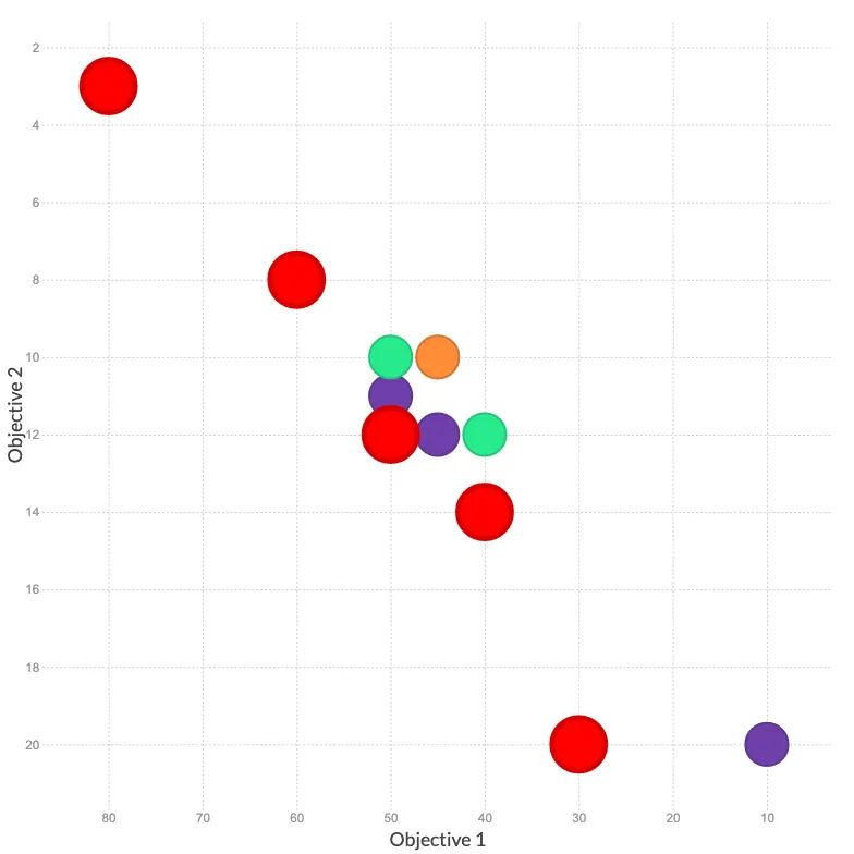
In an earlier section, we briefly covered selection in single-objective problems. There is a fundamental difference between selection in single-objective problems when compared to multi-objective problems. In single-objective problems, we often look for a single solution which has the best objective value, whereas this is not possible in multi-objective problems because they often involve conflicts between multiple objectives. Because multi-objective problems consider more than one objective value, it is often the case that a solution with the best value for one objective will often have degradation in one or more other objective values. This is where a trade-off emerges in the objective space, and it is unlikely that there exists a single solution that can be considered optimal.

Therefore, the solution to a multi-objective optimisation problem is not a single solution vector, but instead an approximation set. This is a set of many candidate solutions that present trade-offs between the multiple objectives, where any improvement in one objective value will result in the degradation in one or more of the other objective values. This notion of "optimum" solutions is called Pareto-optimality.

Pareto-optimality and other approaches to determining dominance relationships between multiple solutions in a population are important during the selection stage of an optimisation algorithm, highlighted below.

Notation

Let's define a multi-objective function $f(x)$ consisting of two objectives.

We have a population $\mathrm{X}$ of $\mathrm{N}$ candidate solutions.

where $\mathrm{N}$ refers to the number of solutions in the population, ${\mathrm{X}}_n$ refers to the $n$-th solution in the population, and $x_{dn}$ refers to the $d$-th decision variable of the $n$-th solution in the population.

We will also define the corresponding objective values $\mathrm{Y}$ which are calculated when evaluating the function in Equation 1.

where $\mathrm{N}$ refers to the number of objective value sets, ${\mathrm{Y}}_n$ refers to the $n$-th set of objective values in the population, and $y_{mn}$ refers to the $m$-th objective value of the $n$-th set of objective values in the population.

Dominance

When using or designing algorithms to solve multi-objective optimisation problems, we will often encounter the concept of domination. This concept is useful for comparing two solutions to determine whether one is better than the other.

We can now use our notation to define dominance relationships. Let's take two solutions to a two-objective problem: ${\mathrm{X}}_1$ and ${\mathrm{X}}_2$, with their corresponding objective values ${\mathrm{Y}}_1=⟨y_{1,1},y_{2,1}⟩$ and ${\mathrm{Y}}_2=⟨y_{1,2},y_{2,2}⟩$.

Definition 1: A solution ${\mathrm{X}}_1$ is said to dominate another solution ${\mathrm{X}}_2$, if both of the following conditions are satisfied:

1. The objective values of ${\mathrm{X}}_1$ are no worse than those of ${\mathrm{X}}_2$ in all objectives, i.e. for this two-objective problem $f_m({\mathrm{X}}_1)\le f_m({\mathrm{X}}_2)$ for all $m=(1,2)$.

2. The objective values of solution ${\mathrm{X}}_1$ are strictly better than at least one of those of solution ${\mathrm{X}}_2$, i.e. for this two-objective problem $f_m({\mathrm{X}}_1)<f_m({\mathrm{X}}_2)$ for at least one $m=(1,2)$.

If any of the two conditions are violated, the solution ${\mathrm{X}}_1$ does not dominate the solution ${\mathrm{X}}_2$ . Otherwise, we can claim ${\mathrm{X}}_1$ dominates ${\mathrm{X}}_2$.

Definition 2: Two solutions ${\mathrm{X}}_1$ and ${\mathrm{X}}_2$ are said to be non-dominating with respect to each other if the following conditions are satisfied:

1. The objective values of solution ${\mathrm{X}}_1$ are strictly better than at least one of those of solution ${\mathrm{X}}_2$, i.e. for this two-objective problem $f_m({\mathrm{X}}_1)<f_m({\mathrm{X}}_2)$ for at least one $m=(1,2)$.

2. The objective values of solution ${\mathrm{X}}_1$ are strictly worse than at least one of those of solution ${\mathrm{X}}_2$, i.e. for this two-objective problem $f_m({\mathrm{X}}_1)>f_m({\mathrm{X}}_2)$ for at least one $m=(1,2)$.

Selecting Solutions

Generally, one of our goals throughout the optimisation process is to select the best solutions. This means that solutions that can be categorised as either "dominating" or "non-dominating" are solutions that we are interested in. To be clear, we are not interested in solutions that are dominated, because they do not offer any desirable performance with respect to any of the considered objectives.

Let's use Python to demonstrate these dominance relations that are often used for selection. Here, we will assume a minimisation problem, where smaller values are better. We will initialise four sets of solutions by synthetically assigning objective values that will demonstrate our dominance relations.

Our first set ${\mathrm{Y}}_1$ and ${\mathrm{Y}}_2$ will demonstrate the scenario where ${\mathrm{Y}}_1$ dominates ${\mathrm{Y}}_2$.

Y1 = np.array([0, 0.5])
Y2 = np.array([0.5, 0.5])

Our second set ${\mathrm{Y}}_3$ and ${\mathrm{Y}}_4$ will demonstrate the scenario where ${\mathrm{Y}}_3$ is identical to ${\mathrm{Y}}_4$.

Y3 = np.array([0.5, 0.5])
Y4 = np.array([0.5, 0.5])

Our third set ${\mathrm{Y}}_5$ and ${\mathrm{Y}}_6$ will demonstrate the scenario where ${\mathrm{Y}}_5$ and ${\mathrm{Y}}_6$ are non-dominated with respect to each other.

Y5 = np.array([0, 0.5])
Y6 = np.array([0.5, 0])

Our fourth set ${\mathrm{Y}}_7$ and ${\mathrm{Y}}_8$ will demonstrate the scenario where ${\mathrm{Y}}_7$ is dominated by ${\mathrm{Y}}_8$.

Y7 = np.array([0.5, 0.5])
Y8 = np.array([0, 0.25])

First, we will define a function to determine whether a solution dominates another or not.

def dominates(X1, X2):
    if np.any(X1 < X2) and np.all(X1 <= X2):
        return True
    else:
        return False

Now, let's test it with our four sets of objective values.

dominates(Y1, Y2)

True

dominates(Y3, Y4)

False

dominates(Y5, Y6)

False

dominates(Y7, Y8)

False

As expected, the only solution pairing that satisfies the criteria for dominance is our first set ${\mathrm{Y}}_1$ and ${\mathrm{Y}}_2$.

Next, let's define a function to determine whether two solutions are non-dominated.

def nondominated(X1, X2):
    if np.any(X1 < X2) and np.any(X1 > X2):
        return True
    else:
        return False

Again, we will test it with our four sets of objective values.

nondominated(Y1, Y2)

False

nondominated(Y3, Y4)

False

nondominated(Y5, Y6)

True

nondominated(Y7, Y8)

False

As expected, the only solution pairing that satisfies the criteria for dominance is our first set ${\mathrm{Y}}_5$ and ${\mathrm{Y}}_6$.

We can string these two functions together within a decision structure to determine the dominance relation between any two solutions.

def dominance_relation(X1, X2):
    if np.all(X1 == X2):
        print("The solutions are identical.")
    elif dominates(X1, X2):
        print("The first solution dominates the second.")
    elif nondominated(X1, X2):
        print("The two solations are nondominating")
    else:
        print("The first solution is dominated by the second.")

Finally, we will test it with our four sets of objective values.

dominance_relation(Y1, Y2)

The first solution dominates the second.

dominance_relation(Y3, Y4)

The solutions are identical.

dominance_relation(Y5, Y6)

The two solations are nondominating

dominance_relation(Y7, Y8)

The first solution is dominated by the second.

Visualisation

Dominance relations can be clearly visualised when working in a two-objective space. Let's do this with some arbitrary solutions. We'll use the ParetoFront visualisation type from PlotAPI.

The figure presents arbitrary solutions to a hypothetical minimisation problem. That is, the lower the values for Objective 1 and Objective 2, the better. PlotAPI ParetoFront has colour-coded the solutions according to their rank, where solutions of the same colour can be considered non-dominated with respect to each other.

Conclusion

In this section we introduced the concept of Pareto-optimality and looked at dominance relations in more detail, complete with examples in Python. The next challenge we will encounter is when we need to select a subset of solutions from a population that consists of entirely non-dominated solutions. For example, which 100 solutions do we select from a population of 200 non-dominated solutions? We will offer some solutions to this challenge in the later sections.