Practical Evolutionary Algorithms
A practical book on Evolutionary Algorithms that teaches you the concepts and how they’re implemented in practice.
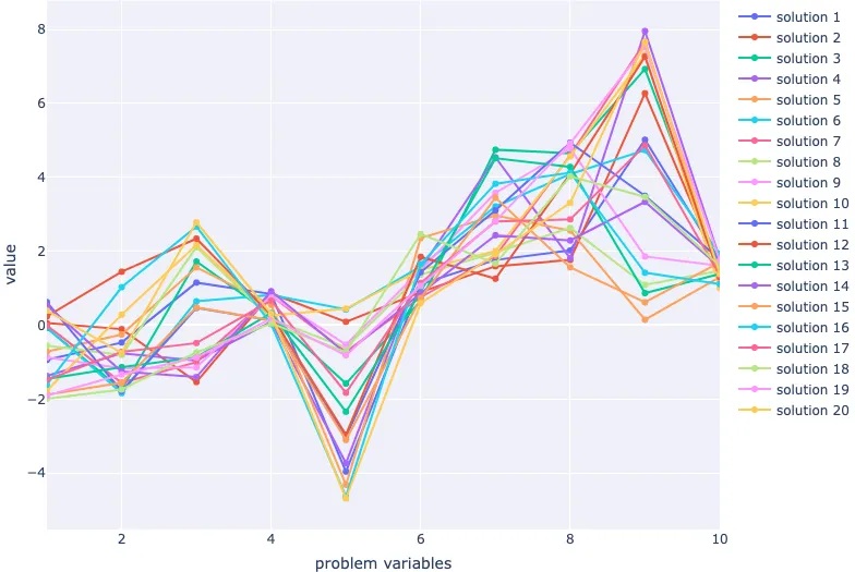
Get the bookpractical evolutionary algorithms Population Initialisation
Before the main optimisation process can begin, we need to complete the initialisation stage of the algorithm. There are many schemes for generating the initial population - let's start simple.

From the collection
Practical Evolutionary Algorithms
A practical book on Evolutionary Algorithms that teaches you the concepts and how they’re implemented in practice.
Get the book
ISBN
978-1-915907-00-4
Cite
Rostami, S. (2020). Practical Evolutionary Algorithms. Polyra Publishing.