Practical Evolutionary Algorithms
A practical book on Evolutionary Algorithms that teaches you the concepts and how they’re implemented in practice.
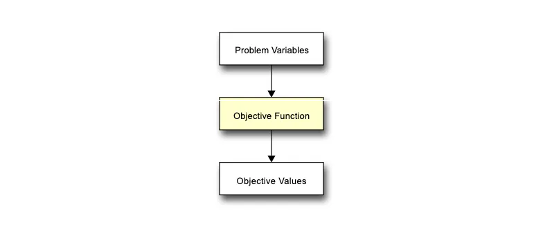
Get the bookpractical evolutionary algorithms Objective Functions
Objective functions are perhaps the most important part of any Evolutionary Algorithm, whilst simultaneously being the least important part too.

From the collection
Practical Evolutionary Algorithms
A practical book on Evolutionary Algorithms that teaches you the concepts and how they’re implemented in practice.
Get the book
ISBN
978-1-915907-00-4
Cite
Rostami, S. (2020). Practical Evolutionary Algorithms. Polyra Publishing.