

Machine Learning
A collection of articles on Machine Learning that teach you the concepts and how they’re implemented in practice.
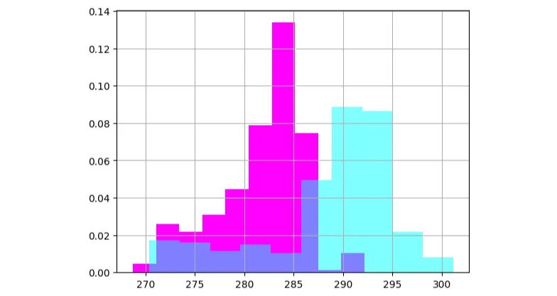
machine learning Pairwise Comparison
Pairwise comparison of data-sets is very important. It allows us to compare two sets of data and make decisions based on the outcome.
- Previous
- Standard Deviation
From the collection
Machine Learning
A collection of articles on Machine Learning that teach you the concepts and how they’re implemented in practice.