Practical Evolutionary Algorithms
A practical book on Evolutionary Algorithms that teaches you the concepts and how they’re implemented in practice.
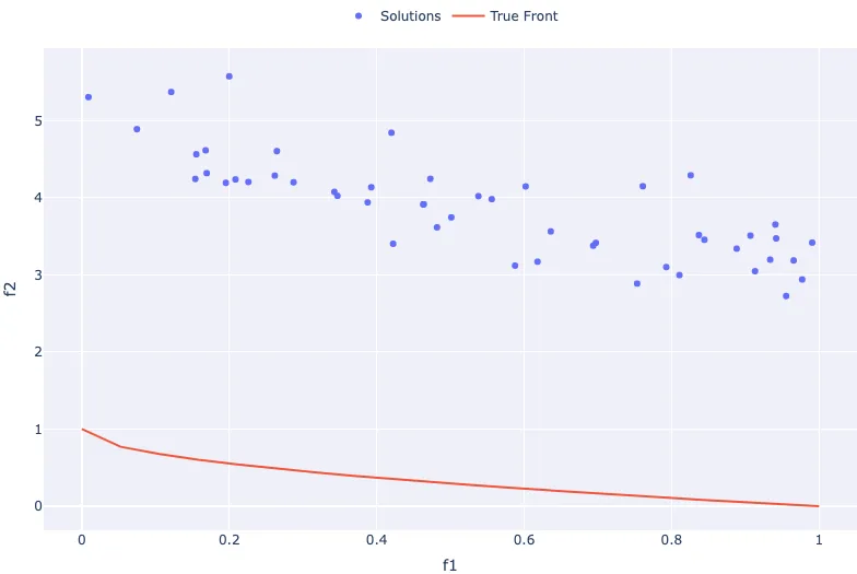
Get the bookpractical evolutionary algorithms Synthetic Objective Functions and ZDT1
We will be using a synthetic test problem throughout this notebook called ZDT1. It is part of the ZDT test suite, consisting of six different two-objective synthetic test problems.

- Previous
- Objective Functions
From the collection
Practical Evolutionary Algorithms
A practical book on Evolutionary Algorithms that teaches you the concepts and how they’re implemented in practice.
Get the book
ISBN
978-1-915907-00-4
Cite
Rostami, S. (2020). Practical Evolutionary Algorithms. Polyra Publishing.