
Get access to this section and more
This is a featured selection from this section. You can access this notebook and more by getting the e-book, Practical Evolutionary Algorithms.
A practical book on Evolutionary Algorithms that teaches you the concepts and how they’re implemented in practice.
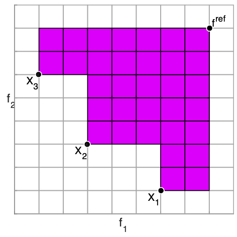
Get the bookThe hypervolume indicator is a performance metric for indicating the quality of a non-dominated approximation set.
Get access to this section and more
This is a featured selection from this section. You can access this notebook and more by getting the e-book, Practical Evolutionary Algorithms.
A practical book on Evolutionary Algorithms that teaches you the concepts and how they’re implemented in practice.
978-1-915907-00-4
Rostami, S. (2020). Practical Evolutionary Algorithms. Polyra Publishing.