Machine Learning
A collection of articles on Machine Learning that teach you the concepts and how they’re implemented in practice.
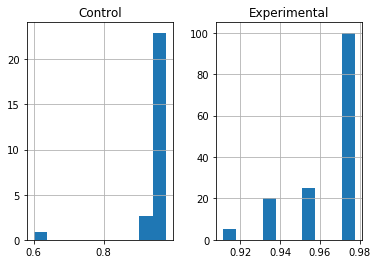
machine learning Results Analysis
Supported by figures and statistics, we will have a look at how our solution performed and discuss anything interesting about the results.

From the collection
Machine Learning
A collection of articles on Machine Learning that teach you the concepts and how they’re implemented in practice.