Machine Learning
A collection of articles on Machine Learning that teach you the concepts and how they’re implemented in practice.
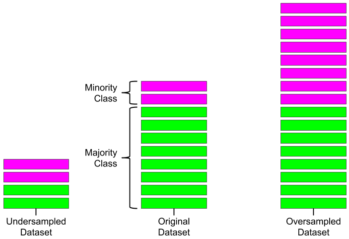
machine learning Class Imbalance and Oversampling
Let's take a quick look at the problem of imbalanced datasets and one way to address it with oversampling.

- Previous
- Results Analysis
From the collection
Machine Learning
A collection of articles on Machine Learning that teach you the concepts and how they’re implemented in practice.