Signal Processing
Signal processing basics and EEG.
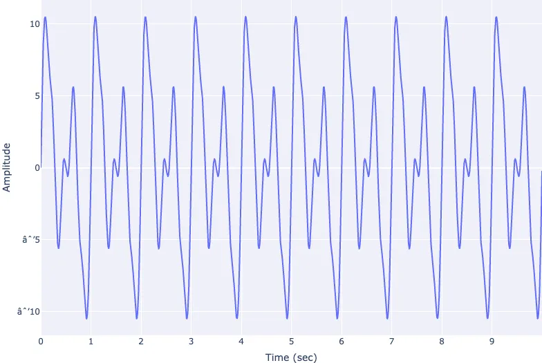
signal processing Summing Sine Waves
We move on from creating and plotting individual sine waves, to summing them and plotting our new and more complicated wave.

From the collection
Signal Processing
Signal processing basics and EEG.