practical evolutionary algorithms Algorithm Performance and Statistical Significance

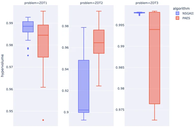
Preamble

import numpy as np                   # for multi-dimensional containers
import pandas as pd                  # for DataFrames
import platypus as plat              # multi-objective optimisation framework
import plotly.express as px
from scipy import stats

Introduction

When preparing to implement multi-objective optimisation experiments, it's often more convenient to use a ready-made framework/library instead of programming everything from scratch. Many libraries and frameworks have been implemented in many different programming languages. With our focus on multi-objective optimisation, our choice is an easy one. We will choose Platypus which has a focus on multi-objective problems and optimisation.

Platypus is a framework for evolutionary computing in Python with a focus on multiobjective evolutionary algorithms (MOEAs). It differs from existing optimization libraries, including PyGMO, Inspyred, DEAP, and Scipy, by providing optimization algorithms and analysis tools for multiobjective optimization.

In this section, we will use the Platypus framework to compare the performance of the Non-dominated Sorting Genetic Algorithm II (NSGA-II)¹ and the Pareto Archived Evolution Strategy (PAES)². To do this, we will use them to generate solutions to three problems in the ZDT test suite³.

Because both of these algorithms are stochastic, meaning that they will produce different results every time they are executed, we will select a sufficient sample size of 30 per algorithm per test problem. We will also use the default configurations for all the test problems and algorithms employed in this comparison. We will use the Hypervolume Indicator (introduced in earlier sections) as our performance metric.

This time, we will also try to test the significance of our results.

Significance testing

Finally, let's test the significance of our pairwise comparison. The significance test you select depends on the nature of your data-set and other criteria, e.g. some select non-parametric tests if their data-sets are not normally distributed. We will use the Wilcoxon signed-rank test through the following function: scipy.stats.wilcoxon():

The Wilcoxon signed-rank test tests the null hypothesis that two related paired samples come from the same distribution. In particular, it tests whether the distribution of the differences x - y is symmetric about zero. It is a non-parametric version of the paired T-test.

https://docs.scipy.org/doc/scipy/reference/generated/scipy.stats.wilcoxon.html

This will give us some idea as to whether the results from one algorithm are significantly different from those from another algorithm.

Executing an Experiment and Generating Results

In this section, we will be using the Platypus implementation of NSGA-II and PAES to generate solutions for the ZDT1, ZDT2, and ZDT3 test problems.

First, we will create a list named problems where each element is a ZDT test problem that we want to use.

problems = [plat.ZDT1, plat.ZDT2, plat.ZDT3]

Similarly, we will create a list named algorithms where each element is an algorithm that we want to compare.

algorithms = [plat.NSGAII, plat.PAES]

Now we can execute an experiment, specifying the number of function evaluations, $nfe=5,000$, and the number of executions per problem, $seed=30$. This may take some time to complete depending on your processor speed and the number of function evaluations.

results = plat.experiment(algorithms, problems, nfe=5000, seeds=30)

Once the above execution has completed, we can initialize an instance of the hypervolume indicator provided by Platypus.

hyp = plat.Hypervolume(minimum=[0, 0], maximum=[11, 11])

Now we can use the calculate function provided by Platypus to calculate all our hypervolume indicator measurements for the results from our above experiment.

hyp_result = plat.calculate(results, hyp)

Finally, we can display these results using the display function provided by Platypus.

plat.display(hyp_result, ndigits=3)

NSGAII
    ZDT1
        Hypervolume : [0.986, 0.99, 0.988, 0.988, 0.986, 0.978, 0.988, 0.982, 0.99, 0.992, 0.984, 0.993, 0.987, 0.975, 0.987, 0.991, 0.991, 0.987, 0.99, 0.992, 0.991, 0.991, 0.989, 0.992, 0.986, 0.979, 0.989, 0.99, 0.99, 0.986]
    ZDT2
        Hypervolume : [0.902, 0.968, 0.965, 0.902, 0.902, 0.901, 0.899, 0.9, 0.927, 0.948, 0.902, 0.901, 0.901, 0.9, 0.898, 0.979, 0.975, 0.9, 0.915, 0.898, 0.9, 0.955, 0.893, 0.902, 0.903, 0.966, 0.895, 0.897, 0.904, 0.959]
    ZDT3
        Hypervolume : [0.998, 0.998, 0.998, 0.998, 0.998, 0.998, 0.998, 0.998, 0.998, 0.998, 0.998, 0.998, 0.998, 0.998, 0.998, 0.998, 0.998, 0.997, 0.998, 0.998, 0.998, 0.998, 0.998, 0.997, 0.998, 0.998, 0.998, 0.998, 0.998, 0.998]
PAES
    ZDT1
        Hypervolume : [0.982, 0.984, 0.987, 0.991, 0.961, 0.97, 0.989, 0.985, 0.992, 0.977, 0.968, 0.975, 0.976, 0.995, 0.987, 0.982, 0.989, 0.961, 0.986, 0.986, 0.983, 0.946, 0.972, 0.994, 0.99, 0.968, 0.985, 0.989, 0.989, 0.976]
    ZDT2
        Hypervolume : [0.992, 0.955, 0.986, 0.952, 0.974, 0.959, 0.944, 0.958, 0.971, 0.994, 0.969, 0.976, 0.956, 0.991, 0.955, 0.924, 0.928, 0.994, 0.97, 0.96, 0.983, 0.94, 0.947, 0.969, 0.928, 0.976, 0.97, 0.957, 0.955, 0.979]
    ZDT3
        Hypervolume : [0.997, 0.998, 0.989, 0.998, 0.987, 0.997, 0.996, 0.976, 0.986, 0.997, 0.998, 0.998, 0.974, 0.998, 0.998, 0.973, 0.976, 0.998, 0.998, 0.976, 0.992, 0.99, 0.976, 0.976, 0.976, 0.978, 0.996, 0.982, 0.998, 0.998]

Statistical Comparison of the Hypervolume Results

Now that we have a data structure that has been populated with results from each execution of the algorithms, we can do a quick statistical comparison to give us some indication as to which algorithm (NSGA-II or PAES) performs better on each problem.

We can see in the output of display above that the data structure is organised as follows:

• Algorithm name (e.g. NSGAII)
  • Problem name (e.g. ZDT1)
    • Performance metric (e.g. Hypervolume)
      • The score for each run (e.g. 30 individual scores).

As a quick test, let's try and get the hypervolume indicator score for the first execution of NSGA-II on ZDT1.

hyp_result["NSGAII"]["ZDT1"]["Hypervolume"][0]

0.9859390491992907

To further demonstrate how this works, let's also get the hypervolume indicator score for the sixth execution of NSGA-II on ZDT1.

hyp_result["NSGAII"]["ZDT1"]["Hypervolume"][5]

0.9782784950959916

Finally, let's get the hypervolume indicator scores for all executions of NSGA-II on ZDT1.

hyp_result["NSGAII"]["ZDT1"]["Hypervolume"]

[0.9859390491992907,
 0.9904112387350754,
 0.9878135459320053,
 0.9882327491808417,
 0.986130505470827,
 0.9782784950959916,
 0.9883480972771655,
 0.9821851637665012,
 0.9897947653205316,
 0.9918251494507012,
 0.9842120139815093,
 0.9926435269821238,
 0.9872816452833134,
 0.9752853822256519,
 0.9866430368587975,
 0.9906683280064335,
 0.9912625719883672,
 0.9874916524247019,
 0.990063965234207,
 0.9919466459035517,
 0.9911540462263884,
 0.990881756200194,
 0.9890600738876908,
 0.992192578855859,
 0.9857010497516153,
 0.9786592166784357,
 0.9887474435457182,
 0.9902866301249156,
 0.9895978887488959,
 0.9855584501975401]

Perfect. Now we can use numpy to calculate the mean hypervolume indicator value for all of our executions of NSGA-II on ZDT1.

np.mean(hyp_result["NSGAII"]["ZDT1"]["Hypervolume"])

0.9876098887511616

Let's do the same for PAES.

np.mean(hyp_result["PAES"]["ZDT1"]["Hypervolume"])

0.9805434942347478

We can see that the mean hypervolume indicator value for PAES on ZDT1 is higher than that of NSGA-II on ZDT1. A higher hypervolume indicator value indicates better performance, so we can tentatively say that PAES outperforms NSGA-II on our configuration of ZDT according to the hypervolume indicator. Of course, we haven't determined if this result is statistically significant.

Let's create a DataFrame where each column refers to the mean hypervolume indicator values for the test problems ZDT1, ZDT2, and ZDT3, and each row represent the performance of an algorithm (in this case, PAES and NSGA-II).

df_hyp_results = pd.DataFrame(index=hyp_result.keys())

for key_algorithm, algorithm in hyp_result.items():
    for key_problem, problem in algorithm.items():
        df_hyp_results.loc[key_algorithm, key_problem] = np.mean(
            problem["Hypervolume"]
        )

df_hyp_results

Now we have an overview of how our selected algorithms performed on the selected test problems according to the hypervolume indicator. It can be easier to compare algorithm performance when each column represents a different algorithm rather than a problem.

df_hyp_results.transpose()

Without consideration for statistical significance, which algorithm performs best on each test problem?

Visualisation

Our results would be better presented with a box plot. Let's wrangle our results from their current data structure, into one that is more suitable for visualisation.

dict_results = []

for key_algorithm, algorithm in hyp_result.items():
    for key_problem, problem in algorithm.items():
        for hypervolume in problem["Hypervolume"]:
            dict_results.append(
                {
                    "algorithm": key_algorithm,
                    "problem": key_problem,
                    "hypervolume": hypervolume,
                }
            )

df_results = pd.DataFrame(dict_results)
df_results

With our data adequately angled, we can produce our visualisation.

fig = px.box(
    df_results,
    facet_col="problem",
    y="hypervolume",
    color="algorithm",
    facet_col_spacing=0.07
)
fig.update_yaxes(matches=None, showticklabels=True)
fig.show()

It's important to understand that these complex algorithms have been implemented many times by different engineers and researchers. The description of complex software and its explanation to a human is a difficult task which can easily lead to misinterpretations⁴. Therefore, it is likely that two implementations of the same algorithm will produce entirely significantly different performance profiles.

Significance Testing

Now let's use the Wilcoxon signed-rank test that we introduced above to see if our results are significant, or if any difference in observation occurred purely by chance.

Before using the test, we need to decide on a value for alpha, our significance level. This is essentially the “risk” of concluding a difference exists when it doesn’t, e.g., an alpha of $0.05$ indicates a 5% risk. We can consider alpha to be some kind of threshold. This will be covered in more detail in another article, but for now, we will set $0.05$ as our alpha. This means if our p-value is less than $0.05$, the null hypothesis has been rejected and the samples are likely not from the same distribution. Otherwise, the null hypothesis cannot be rejected, and the samples are likely from the same distribution.

We will use NSGA-II as our benchmark algorithm, meaning we will compare every other algorithm that we're considering to NSGA-II to determine if the results were significant. Let's write some code to determine this for us:

algorithms = ['NSGAII', 'PAES']
problems = ['ZDT1', 'ZDT2', 'ZDT3']


df_hyp_wilcoxon = pd.DataFrame(index = [algorithms[1]])


for key_problem in problems:
    s, p = stats.wilcoxon(hyp_result[algorithms[0]][key_problem]['Hypervolume'],
                          hyp_result[algorithms[1]][key_problem]['Hypervolume'])
    df_hyp_wilcoxon.loc[algorithms[1],key_problem] = p
            
df_hyp_wilcoxon.transpose()

We can see that in every case, $p<0.05$. Therefore according to our configuration of $alpha$, our results are statistically significant. Looking back at the mean hypervolume results:

df_hyp_results.transpose()

With respect to hypervolume indicator quality, we can now say that:

• NSGA-II outperforms PAES on ZDT1.
• PAES outperforms NSGA-II on ZDT2.
• NSGA-II outperforms PAES on ZDT3.

The results are statistically significant.

Conclusion

In this section, we have demonstrated how we can compare two popular multi-objective evolutionary algorithms on a selection of three test problems using the hypervolume indicator to measure their performance. In this case, we have also determined the significance of our results using the Wilcoxon signed-rank test.