practical evolutionary algorithms Single Objective Problems

Preamble

import numpy as np                   # for multi-dimensional containers
import pandas as pd                  # for DataFrames
import plotly.graph_objects as go    # for data visualisation

Introduction

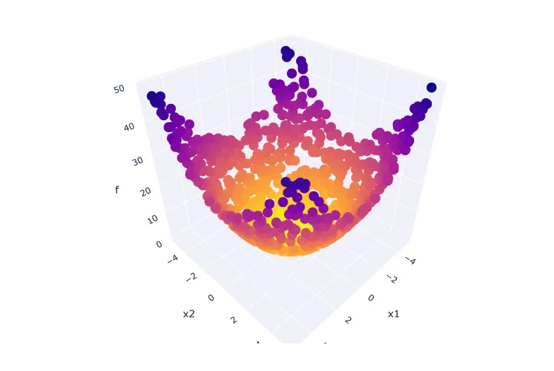
Before moving on, let's take some time to have a closer look at a single-objective problem. This will give us some perspective. In single-objective problems, the objective is to find a single solution which represents the global optimum in the entire search space. Determining which solutions outperform others is a simple task when only considering a single-objective because the best solution is simply the one with the highest (for maximisation problems) or lowest (for minimisation problems) objective value. Let's take the Sphere function as an example.

The Sphere Function

This is a single-objective test function which has been expressed in Equation 1.

where $x_d\in [-5.12,5.12]$, i.e. each problem variable should be between $-5.12$ and $5.12$. It is continuous, convex, and unimodal. It is scalable with regards to its dimensionality in the problem domain, however, we will use its two-dimensional configuration for easy visualisation throughout this notebook. Let's implement this problem in Python so we can evaluate some solutions.

def sphere(x):
    y = np.sum(np.square(x))
    return y

Now let's prepare for the initialisation of five solutions with two problem variables. We will specify the desired population size, $\mathrm{N}$, and the dimensionality of the problem domain, $\mathrm{D}$. We will also specify the lower and upper boundaries for our problem variables.

N = 5
D = 2
D_lower = np.ones((1, D)) * -5.12
D_upper = np.ones((1, D)) * 5.12

Let's initialise a population with random decision variables.

X = pd.DataFrame(np.random.uniform(low=D_lower, high=D_upper, size=(N, D)))
X

To generate $\mathrm{Y}$, we will evaluate each solution ${\mathrm{X}}_{\mathrm{N}}$ using the sphere() test function defined above.

Y = np.empty((0, 1))

X = pd.DataFrame(np.random.uniform(low=D_lower, high=D_upper, size=(N, D)))

for n in range(N):
    y = sphere(X.iloc[n])
    Y = np.vstack([Y, y])

# convert to DataFrame
Y = pd.DataFrame(Y, columns=["f"])

We only have five solutions, so it's feasible to list all our objective values.

Y

We can very easily select the best solution from the above population. It is simply the solution with the smallest objective value (as we are concerned with minimisation).

np.min(Y)

f    1.5598
dtype: float64

Let's see if we can get a better understanding of the problem domain by generating and visualising 1000 more solutions. This means setting $\mathrm{N}=1000$. We can achieve this by repeating the same code as above with slightly different parameters to generate our population of solutions, and then evaluate them using our sphere() function.

N = 1000

X = pd.DataFrame(
    np.random.uniform(low=D_lower, high=D_upper, size=(N, D)),
    columns=["x1", "x2"],
)

Y = np.empty((0, 1))

for n in range(N):
    y = sphere(X.iloc[n])
    Y = np.vstack([Y, y])

Y = pd.DataFrame(Y, columns=["f"])

All that's left now is to visualise the results. For this, we'll use a 3D scatterplot to plot the problem variables of each solution along with each corresponding objective value. We will reserve the vertical axis for the objective value, $f$, meaning that "lower" points represent better performing solutions.

fig = go.Figure(
    layout=dict(
        scene=dict(xaxis_title="x1", yaxis_title="x2", zaxis_title="f")
    )
)

fig.add_scatter3d(
    x=X.x1, y=X.x2, z=Y.f, mode="markers", marker=dict(color=-Y.f)
)

fig.show()

Conclusion

In this section, we covered the very basics on the topic of single-objective optimisation problems using the popular Sphere function as an example. The most important lesson from this section is that it is trivial to determine which solution outperforms the rest when working with a single-objective problem.

In the next section, we will demonstrate why this is more difficult for multi-objective problems, and introduce some approaches to selection.