Data Analysis with Rust Notebooks
A practical book on Data Analysis with Rust Notebooks that teaches you the concepts and how they’re implemented in practice.
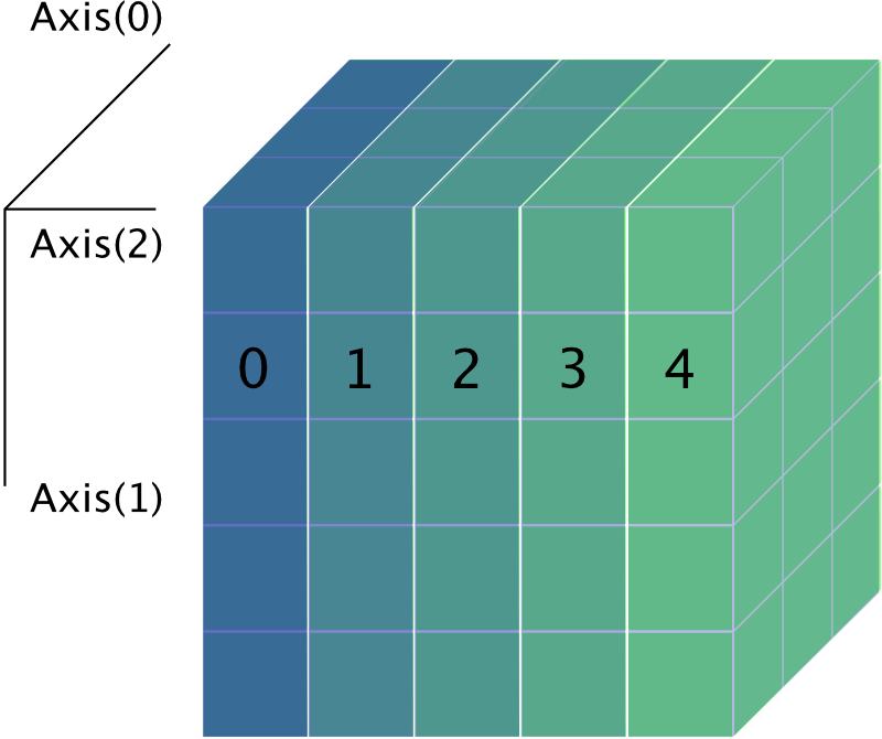
Get the bookdata analysis with rust notebooks Multidimensional Arrays and Operations with NDArray
The ndarray crate provides us with a multidimensional container that can contain general or numerical elements.

From the collection
Data Analysis with Rust Notebooks
A practical book on Data Analysis with Rust Notebooks that teaches you the concepts and how they’re implemented in practice.
Get the book
ISBN
978-1-915907-10-3
Cite
Rostami, S. (2020). Data Analysis with Rust Notebooks. Polyra Publishing.