machine learning Experimental Design

Overview

This will be the second article in a four part series covering the following:

1. Dataset analysis - We will present and discuss a dataset selected for our machine learning experiment. This will include some analysis and visualisations to give us a better understanding of what we 're dealing with.
2. Experimental design - Before we conduct our experiment, we need to have a clear idea of what we 're doing. It's important to know what we're looking for, how we're going to use our dataset, what algorithms we will be employing, and how we will determine whether the performance of our approach is successful.
3. Implementation - We will use the Keras API on top of TensorFlow to implement our experiment. All code will be in Python, and at the time of publishing everything is guaranteed to work within a Kaggle Notebook.
4. Results - Supported by figures and statistics, we will have a look at how our solution performed, and discuss anything interesting about the results.

Experimental design

In the last article we introduced and analysed the Iris Flower Dataset within a Kaggle Kernel notebook. In this article we will design our experiments, and select some algorithms and performance measures to support our implementation and discussion of the results.

A parallel coordinate plot of our dataset grouped by Species.

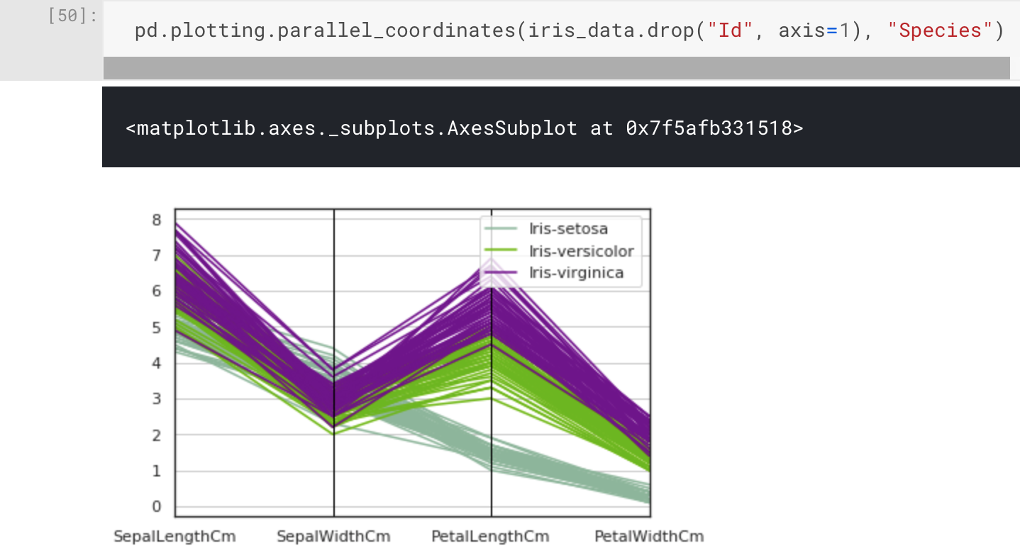
Before moving onto the application of machine learning algorithms, we first need to design our experiment. Doing so will give us a clear idea of what we're looking for, how we intend to get there, and how we will decide the outcome. This process helps us when reporting our findings, whether it's to your stakeholders or a peer-reviewed paper.

This series is aimed at beginners, and we know the Iris Flower dataset is an easy one, so we will keep our idea simple. Let's design an experiment to find out whether the same machine learning algorithm will offer significantly different performance, if we change just one part of the algorithm's configuration. The task we want the solution to complete is multi-class classification, i.e. classifying an Iris Flower dataset sample into one of the three species. In this context, each one of the species can also be referred to as a class.

Algorithm selection

Selecting the right algorithm or set of algorithms for an experiment is often a non-trivial task. However, for this easy problem there is little that is unknown, so we can select something simple without much consideration. For our purposes we will select an Artificial Neural Network learning algorithm, with one criterion: that it is easy to implement using Keras. Keras is the software library we will be using through Python, to code up and conduct our experiments - more on this in the next article.

We will cover Artificial Neural Networks in a different article, but for now let's treat them as a black box , which we will refer to as neural network from now on. Put simply, they are networks of interconnected nodes arranged into layers. A neural network can be used for classification, regression, and clustering. This means it fits our requirement to classify our samples. When pass in our four input parameters (sepal length and width, petal length and width), we will expect an output of either Setosa, Versicolour, or Virginica.

Our black box neural network for classifying Iris Flower dataset samples into one of the three species.

Before our neural network can classify the inputs into what it thinks is the right output, it needs to be trained. Training usually involves adapting the strength of the connections between nodes within a neural network, often referred to as the weights. By continuously adapting these weights, which are used in calculations involving the input samples, a learning algorithm can try to learn the classification problem. The desirable output is a classifier that can map input samples to the desired/correct output.

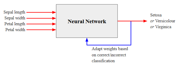
Many variables effect the performance, e.g. in terms of accuracy, of a neural network classifier, these include:

• Topology/Structure:
• Number of Hidden Layers
• Number of Neurons per Hidden Layer
• Trained Parameters:
• Connection Weights
• Neuron Biases

The above is not an exhaustive list, but let's visualise these variables.

An illustration of a feed-forward neural network classifier. Where $x_1\dots x_4$ are the input parameters for a single sample, $w_1\dots w_n$ are the weights, $b_1\dots b_n$ and $a_1\dots a_n$ are the biases and activation functions respectively, and $y_1\dots y_3$ are the outputs.

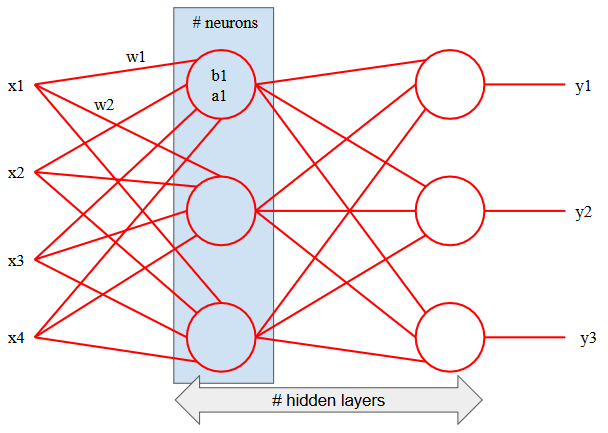
In the above figure we have peered into our black box, and we can see there are four inputs labelled $x_1$ to $x_4$ , 2 hidden layers each with 3 neurons, and three outputs labelled $y_1$ to $y_3$. To keep things simple, we will only use a neural network with a single hidden layer in our experiments.

Scientific control

There are no hard or fast rules for defining the structure of a neural network. However, a general piece of advice is that you should have at least the same number of neurons on a hidden layer as you do on the input layer. This means for our Iris Flower dataset; our hidden layer should consist of four neurons. We will aim to create a neural network with this structure and use the default configurations provided by Keras for everything else. This will be the control arm of our experiment. We will then train the neural network and measure its performance.

We will then run the same experiment again, however this time we will change a single configuration related to the structure of the neural network. We will change the number of hidden layer neurons from four, to five. This will be our experimental arm. This is a controlled experiment, and by only changing one variable we aim to eliminate any other explanations for why the two arms of our experiment perform differently. When analysing our results, we want to be able to say with some confidence: "changing the number of neurons on the hidden layer made a significant difference to the performance of our neural network", and then perhaps observations around which classifier performs better.

Testable hypotheses

Let's define a testable hypothesis. Our hypothesis is a proposed explanation made on the basis of some limited or preliminary evidence, and this will be a starting point for further investigation. We should phrase it such that it is testable, and not ambiguous.

Hypothesis : A neural network classifier's performance on the Iris Flower dataset is affected by the number of hidden layer neurons.

When we test our hypothesis, there are two possible outcomes:

• $H_0$ the null hypothesis : insufficient evidence to support hypothesis.

• $H_1$ the alternate hypothesis : evidence suggests the hypothesis is likely true.

If the null hypothesis is accepted, meaning there's not enough evidence to support our hypothesis, it suggests that there is no significant difference in performance when changing the number of hidden layer neurons. However, if we reject the null hypothesis and accept the alternate hypothesis, this suggests that it is likely there's a significant difference in performance when changing the number of hidden layer neurons.

Sample size sufficiency

Neural network training algorithms are stochastic, and what this means is that they employ random numbers. One step that often employs random numbers is the initialisation of weights, which when optimised using some training algorithm will offer different performance every time. This often catches beginners out, and must be taken into consideration when designing an experiment.

To demonstrate, I went ahead and set up a neural network within Keras with default configurations, and a single hidden layer consisting of 12 neurons. I executed the same code 10 individual times, and here are the accuracy results:

Accuracy
0.9777777777777777
0.9888888888888889
0.9555555489328172
0.9888888809416029
0.9666666666666667
1.0
0.9888888809416029
0.9888888888888889
0.9777777791023254
0.9666666666666667

As we can see from these preliminary results, the same algorithm with identical configuration has produced 10 different classifiers which all offer varying performance. By chance, some of the executions have produced classifiers which have reported the same performance as others, but these are likely to have entirely different weights. There is a way to get around this and always reproduce an identical neural network classifier, and that's by using the same seed for your random number generators. However, this doesn't tell us how good an algorithm is at training a neural network.

The real solution is to determine a sufficient sample size for your experiment. In this context, we're referring to each execution of your algorithm as a sample, and not the samples within the dataset as we were previously. There are many methods to determine a sufficient sample size, however, for the purpose of this series we will simply select a sample size of 30, which is a number often selected in the literature. This means we will be executing each algorithm 30 times, and then using some statistics to determine performance.

Significance testing

Now that we are comparing a population of 30 performance measures per arm of our experiment, instead of just a reading, we will need to rely on something like mean average of both arms to measure a difference or if one outperforms the other. However, the mean average alone is not enough evidence to reject the null hypothesis. Along with a sufficient sample size, we need to determine whether we need to run a parametric or non-parametric test. These tests should give us an indication of whether any difference between our two sets of results was "significant" or "by chance".

Simple steps for a pairwise comparison of machine learning results.

Parametric tests typically work well on sets that follow a normal distribution, and non-parametric tests typically work well on sets that don't. This is a topic we'll visit in a different article in the future, but for now we will select a non-parametric test called the Wilcoxon Rank Sums test.

This test aligns with our hypothesis, as it is used to determine whether two set of samples come from different distributions. Through this test, we can find out if it's likely or not that there's a significant difference between our two experiment arms.

Training and Testing Strategy

We need to decide on how we're going to use our data to train and then test our models. The easiest way is to divide the dataset samples into a training set and testing set, often in an 80-20 split. The training samples will be used by the learning algorithms to find the optimal weights. The testing set is used only to assess the performance of a fully-trained model, and must remain entirely unseen by the learning algorithm. The test set can be seen as a portion of the dataset which is kept in a "vault" until the very end. After assessing the model with the testing set, there can be no further tuning unless there are new and unseen samples which can be used for testing.

A simple training and testing strategy.

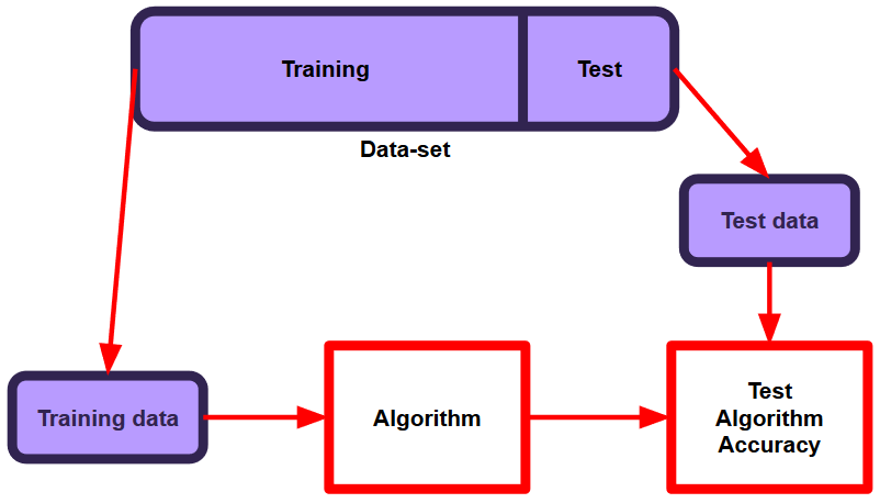
The Iris Flower dataset is relatively small at exactly 150 samples. Because of this, we will use 70% of the dataset for training, and the remaining 30% for testing, otherwise our test set will be a little on the small side.

Performance Evaluation

Let's decide on how we will evaluate the performance of our experiments, and how we will interpret the results. First, let's define what we mean by true positives, false positives, true negatives, and false negatives, as these are used in the calculations for many of the popular metrics.

After a neural network has been trained using the training set, its predictive performance is tested using the test set. Through this exercise, we are able to see if the classifier was able to correctly classify each sample. In a binary classification problem where the output can only be true or false, we can use something called the confusion matrix:

A confusion matrix can be used to present the number of samples that were correctly or incorrectly classified.

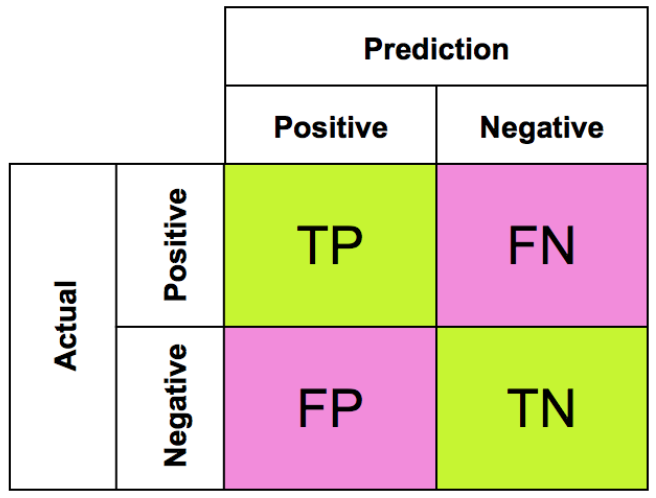
True Positive (TP) - belong to the positive class and were correctly classified as the positive class.

False Positive (FP) - belong to the negative class and were incorrectly classified as the positive class.

True Negative (TN) - belong to the negative class and were correctly classified as the negative class.

False Negative (FN) - belong to the positive class and were incorrectly classified as the negative class.

However, in a multi-class classification problem the confusion matrix would look more like the following:

A simple Hello World program written in Python within a Kaggle Notebook.

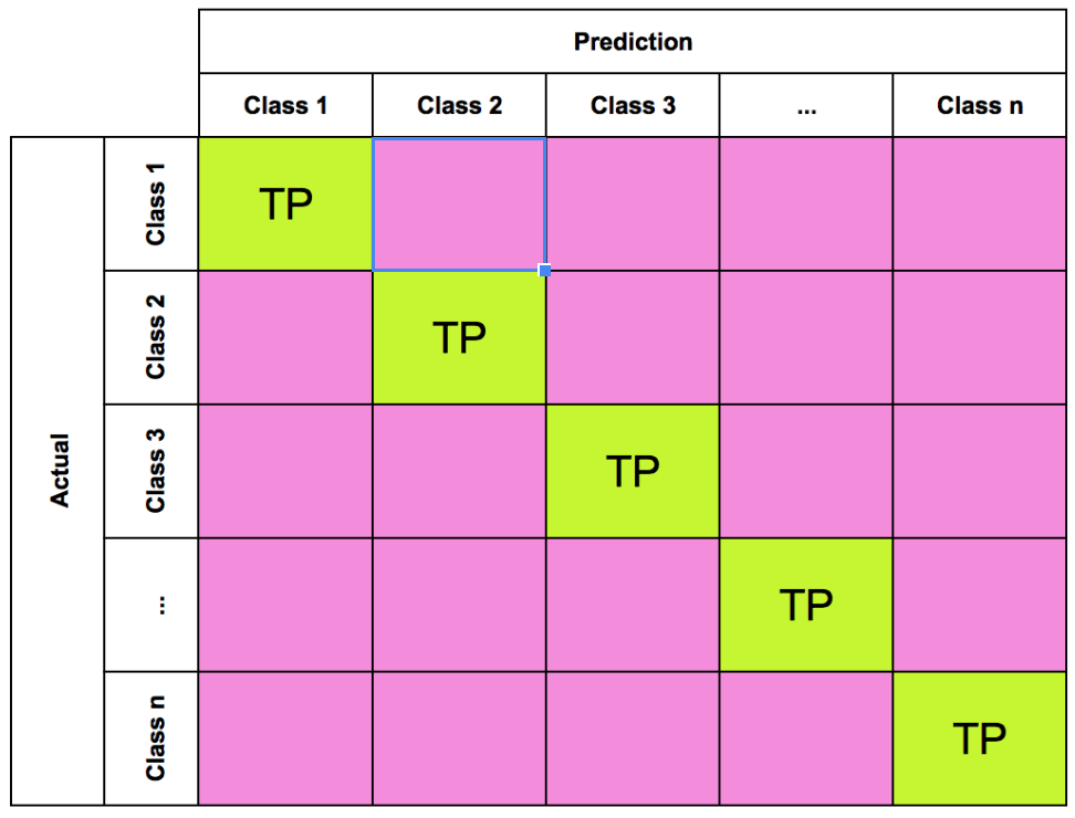
From these counts, we can calculate the following measures:

Accuracy - The percentage of samples correctly identified:

Precision (Positive predictive value) - proportion of positives accurately identified:

Recall (Sensitivity, True Positive Rate) - Proportion of positives correctly identified:

True negative rate (Specificity) - Proportion of negatives correctly identified:

F-measure - Balance between precision and recall:

These metrics all have their uses and are often used in combination to determine the performance of a classifier. The Iris Flower dataset is simple enough for us to use the classification accuracy as our measurement for pairwise comparison. This means for each arm of the experiment, we will complete 30 independent executions and build a set of classification accuracies, and use the mean average and significance testing to check our hypothesis. In addition, we will also report on the above metrics to see how they work.

Conclusion

In this article we've covered a breadth of experimental design issues. We have selected a simple neural network for our experiment, with the control and experiment arm only differing by one neuron on the hidden layer. We discussed the importance of using a sufficient sample size and conducting significance testing, and strategies for splitting the dataset for training and testing. Finally, we decided how we were going to measure our experiment and how we would report the results.

In the next part of this four part series, we will write all the code for the experiments using Python and the Keras API on top of TensorFlow, and collect our results in preparation for the final discussion.