data analysis with rust notebooks Setup Anaconda, Jupyter, and Rust

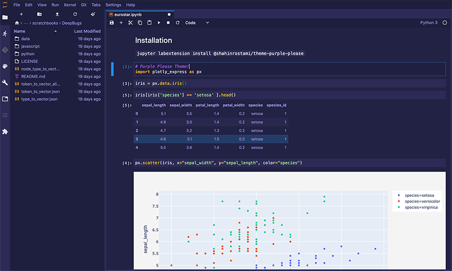
We are taking a practical approach in the following sections. As such, we need the right tools and environments available in order to keep up with the examples and exercises. We will be using Rust along with packages that will form our scientific stack, such as ndarray (for multi-dimensional containers) and plotly (for interactive graphing), etc. We will write all of our code within a Jupyter Notebook, but you are free to use other IDEs.

Install Miniconda

There are many different ways to get up and running with an environment that will facilitate our work. One approach I can recommend is to install and use Miniconda.

Miniconda is a free minimal installer for conda. It is a small, bootstrap version of Anaconda that includes only conda, Python, the packages they depend on, and a small number of other useful packages, including pip, zlib and a few others.

— https://docs.conda.io/en/latest/miniconda.html

You can skip Miniconda entirely if you prefer and install Jupyter Lab directly, however, I prefer using it to manage other environments too.

You can find installation instructions for Miniconda on their website, but if you're using Linux (e.g. Ubuntu) you can execute the following commands from in your terminal:

wget https://repo.continuum.io/miniconda/Miniconda3-latest-Linux-x86_64.sh
chmod +x Miniconda3-latest-Linux-x86_64.sh
./Miniconda3-latest-Linux-x86_64.sh

This will download the installation files and start the interactive installation process. Follow the process to the end, where you should see the following message:

Thank you for installing Miniconda3!

All that's left is to close and re-open the terminal window.

Create Your Environment

Once Miniconda is installed, we need to create and configure our environment. If you added Miniconda to your PATH environment during the installation process, then you can run these commands directly from Terminal, Powershell, or CMD.

Now we can create and configure our conda environment using the following commands.

conda create -n darn python=3

You can replace darn (Data Analytics with Rust Notebooks) with a name of your choosing.

This will create a conda environment named darn with the latest Python 3 package ready to go. You should be presented with a list of packages that will be installed and asked if you wish to proceed. To do so, just enter the character y. If this operation is successful, you should see the following output at the end:

Preparing transaction: done
Verifying transaction: done
Executing transaction: done
#
# To activate this environment, use
#
#     $ conda activate darn
#
# To deactivate an active environment, use
#
#     $ conda deactivate

As the message suggests, you will need to type the following command to activate and start entering commands within our environment named darn.

conda activate darn

Once you do that, you should see your terminal prompt now leads with the environment name within parentheses:

(darn) melica:~ shahin$ 

This will allow you to identify which environment you are currently operating in. If you restart your machine, you should be able to use conda activate darn within your conda prompt to get back into the same environment.

Install Packages

If your environment was already configured and ready, you would be able to enter the command jupyter lab to launch an instance of the Jupyter Lab IDE in the current directory. However, if we try that in our newly created environment, we will receive an error:

(darn) melica:~ shahin$ jupyter lab
-bash: jupyter: command not found

So let's fix that. Let's install Jupyter Lab and use the -y option which automatically says "yes" to any questions asked during the installation process.

conda install -c conda-forge jupyterlab=2.2.9

We'll also need cmake later on.

conda install -c anaconda cmake -y

Finally, let's install nodejs. This is needed to run our Jupyter Lab extension in the next section.

conda install -c conda-forge nodejs=15 -y

Install Jupyer Lab Extensions

There's one last thing we need to do before we move on, and that's installing any Jupyter Lab extensions that we may need. One particular extension that we need is the plotly extension, which will allow our Jupyter Notebooks to render our Plotly visualisations. Within your conda environment, simply run the following command:

jupyter labextension install jupyterlab-plotly

This may take some time, especially when it builds your jupyterlab assets, so keep an eye on it until you're returned control over the conda prompt, i.e. when you see the following:

(darn) melica:~ shahin$ 

Optionally, you may wish to install the purple looking theme from Figure 1 above.

jupyter labextension install @shahinrostami/theme-purple-please

Now we're good to go!

Install Rust

Now we'll install Rust using rustup, but you can check out the other installation methods if you need them.

curl --proto '=https' --tlsv1.2 -sSf https://sh.rustup.rs | sh

The code samples in this book will work in many versions of Rust, but I can confirm them to be working with version 1.42.0. You can get the same version with:

rustup default 1.42.0

You will be given instructions for adding Cargo's bin directory to your PATH environment variable.

source $HOME/.cargo/env

This will work until your close your terminal, so make sure to add it to your shell profile. I use Z shell (Zsh) so this meant adding the following to .zshrc:

export PATH="$HOME/.cargo/bin:$PATH"

You can make sure everything works by closing and re-opening your terminal and typing cargo. If this returns the usage documentation then you're all set.

Install the EvCxR Jupyter Kernel

Now we'll install the EvCxR Jupyter Kernel. If you're wondering how it's pronounced, it's been mentioned to be "Evic-ser". This is what will allow us to execute Rust code in a Jupyter Notebook.

You can get other installation methods methods for EvCxR if you need then, but we will be using:

cargo install evcxr_jupyter --version 0.5.3
evcxr_jupyter --install

A Quick Test

Let's test if everything is working as it should be. In your conda prompt, within your conda environment, run the following command

jupyter lab

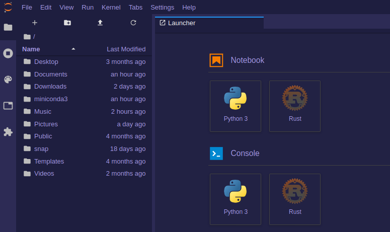
This should start the Jupyter Lab server and launch a browser window with the IDE ready to use.

Let's create a new notebook. In the Launcher tab which has opened by default, click "Rust" under the Notebook heading. This will create a new and empty notebook named Untitled.ipynb in the current directory.

If everything is configured as it should be, you should see no errors. Type the following into the first cell and click the "play" button to execute it and create a new cell.

println!("Hello World!");

Hello World!

If we followed all the instructions and didn't encounter any errors, everything should be working. We should see "Hello World!" in the output cell.

Conclusion

In this section, we've downloaded, installed, configured, and tested our environment such that we're ready to run the following examples and experiments. If you ever find that you're missing Jupyter Lab packages, you can install them in the same way as we installed Jupyter Lab and the others in this section.