Signal Processing
Signal processing basics and EEG.
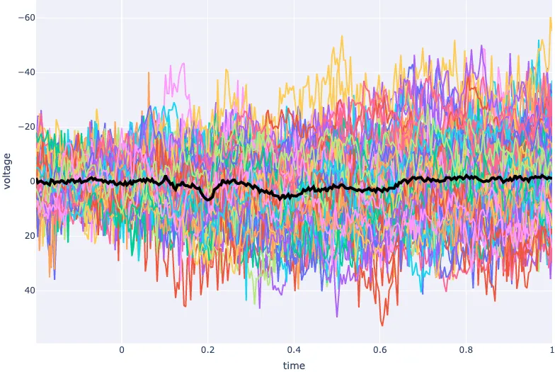
signal processing Time Domain Analysis with Plotly
Plotting multiple channels in the time domain with Plotly.

- Previous
- Time Domain Analysis
From the collection
Signal Processing
Signal processing basics and EEG.