Signal Processing
Signal processing basics and EEG.
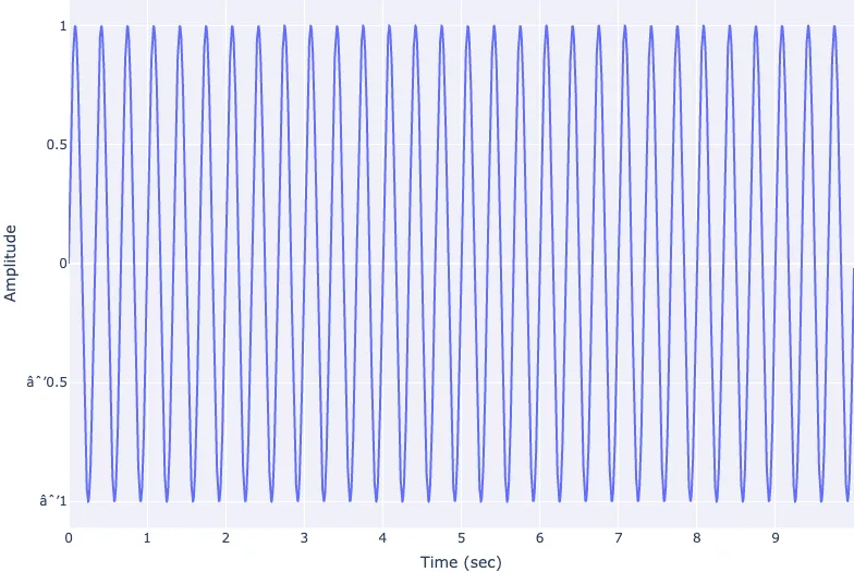
signal processing Sine Waves in the Time Domain
Let's look at a simple sine wave, how to create one in Python and how to visualise it in the time domain using a line chart.

From the collection
Signal Processing
Signal processing basics and EEG.