
Get access to this section and more
This is a featured selection from this section. You can access this notebook and more by getting the e-book, Data Analysis with Rust Notebooks.
A practical book on Data Analysis with Rust Notebooks that teaches you the concepts and how they’re implemented in practice.
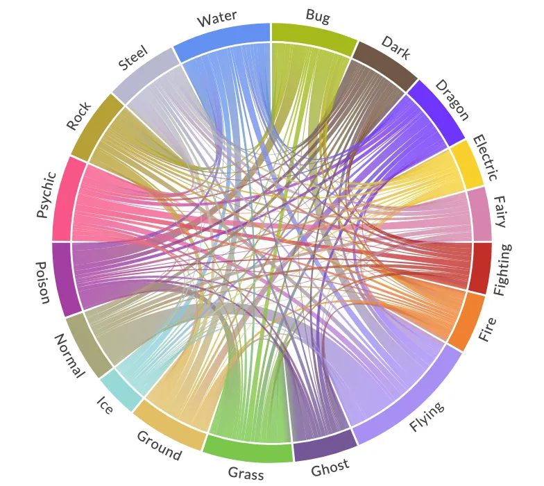
Get the bookWe're going to use the Complete Pokemon Dataset dataset to visualise the co-occurrence of Pokémon types from generations one to eight. We'll make this happen using a chord diagram.
Get access to this section and more
This is a featured selection from this section. You can access this notebook and more by getting the e-book, Data Analysis with Rust Notebooks.
A practical book on Data Analysis with Rust Notebooks that teaches you the concepts and how they’re implemented in practice.
978-1-915907-10-3
Rostami, S. (2020). Data Analysis with Rust Notebooks. Polyra Publishing.