machine learning Standard Deviation

This is a brief re-cap on calculating the standard deviation.

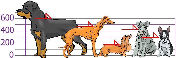
Let's assume that we have measured the height of each member in our population below:

We'll put these in a numpy array so we can use them later on:

import numpy as np
heights = np.array([600, 470, 170, 430, 300])

Calculating the standard deviation with numpy

Numpy has many useful built-in functions. One of these calculates the standard deviation for any set of data, below you can see this in action:

print("standard deviation is {}".format(np.std(heights)))

standard deviation is 147.32277488562318

Calculating the standard deviation ourselves

As always, it's recommended you use these well-maintained functions instead of writing your own. However, with this population size being so small, we can get a better understanding of how the standard deviation is calculated if we do it ourselves.

Let's have a look at the formula:

To those of you who aren't comfortable with mathematics, this can be overwhelming. But let's break it down and calculate everything step-by-step:

First we want to find $\mu$ which is just the mean of the population values. The mean is just all the values summed together and then divided by the population size. For our population, this would be:

population_mean = np.sum(heights) / heights.size
print("population mean is: {}".format(population_mean))

population mean is: 394.0

We can find the mean using a built-in numpy function too:

population_mean = np.mean(heights)
print("population mean is: {}".format(population_mean))

population mean is: 394.0

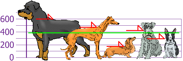
Great - now we have the mean, let's plot it on our graph in green:

Now we want to calculate $(x-\mu )$, which is difference between each height and the mean:

In Python + numpy, we can calculate this:

height_differences = heights - population_mean
print("height differences: {}".format(height_differences))

height differences: [ 206.   76. -224.   36.  -94.]

Now to get the variance which is this part:

To do this, we first square all our height differences above, and get the average of them.

variance = (height_differences**2) 
variance = np.sum(variance)
variance = variance / height_differences.size
print("variance: {}".format(variance))

variance: 21704.0

Again, we can find the variance using a built-in numpy function too:

variance = np.var(height_differences)
print("variance: {}".format(variance))

variance: 21704.0

Finally, the last part is to find the square root of our variance, which is the standard deviation:

standard_deviation = np.sqrt(variance)
print("standard deviation is {}".format(standard_deviation))

standard deviation is 147.32277488562318

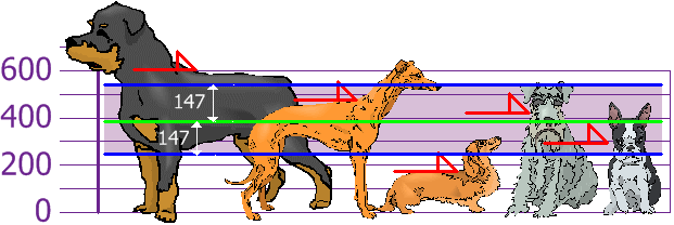
When we plot this standard deviation on our graph we get the following:

With the standard deviation, we can suggest which heights are within our standard deviation (147mm) of the mean. So now there's an approach to knowing what is normal, what is extra large, or extra small.

Population vs Sample

If there data we're working with is a sample taken from a larger population, then there's a slight difference in calculating the standard deviation.

Instead of:

We use:

where $\overline{x}$ is just the sample mean, and $n-1$ is the sample size minus 1.