Data is Beautiful
A practical book on data visualisation that shows you how to create static and interactive visualisations that are engaging and beautiful.
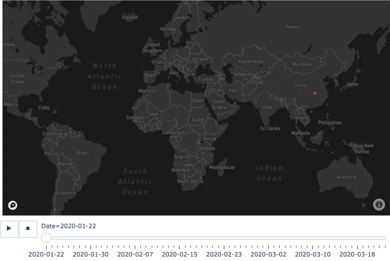
Get the bookdata is beautiful Coronavirus Time Series Map Animation
Coronavirus Time Series Map Animation

From the collection
Data is Beautiful
A practical book on data visualisation that shows you how to create static and interactive visualisations that are engaging and beautiful.