
Preamble
import numpy as np                   # for multi-dimensional containers
import pandas as pd                  # for DataFrames
import plotly.graph_objects as go    # for data visualisation
from plotly.subplots import make_subplots
Creating Sine Waves
In a previous section we looked at how to create a single Sine Wave and visualise it in the time domain.
sample_rate = 1000
start_time = 0
end_time = 10

time = np.arange(start_time, end_time, 1/sample_rate)

frequency = 3
amplitude = 1
theta = 0

sinewave = amplitude * np.sin(2 * np.pi * frequency * time + theta)

fig = go.Figure(layout=dict(xaxis=dict(title='Time (sec)'),yaxis=dict(title='Amplitude')))
fig.add_scatter(x=time, y=sinewave)
fig.show()
Creating Multiple Sine Wave
Let's create and plot five sine waves. Let's start by defining our time window and sample rate.
sample_rate = 1000
start_time = 0
end_time = 10
theta = 0

time = np.arange(start_time, end_time, 1/sample_rate)
Now we'll store their frequencies in a list named frequency, and their amplitudes in a list named amplitude.
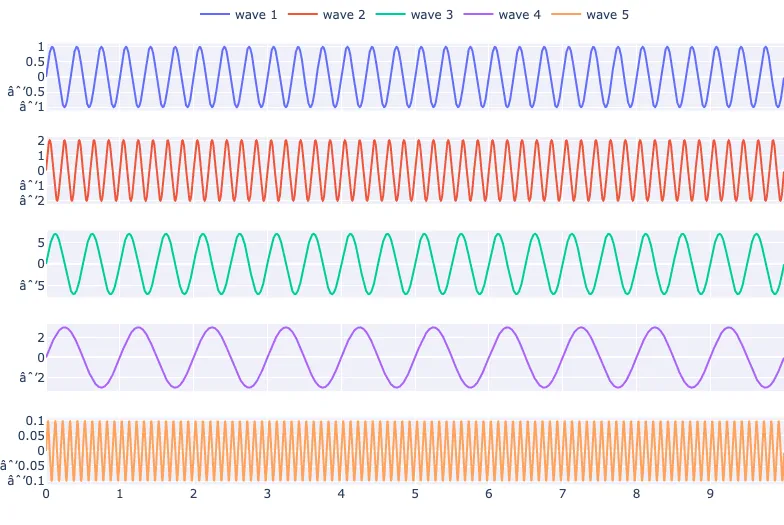
frequency = [3, 5, 2, 1, 10]
amplitude = [1, 2, 7, 3, 0.1]
Finally, let's loop through our five frequency/amplitude values and use them to calculate and visualise the sine waves using subplots.
fig = make_subplots(rows=5, cols=1, shared_xaxes=True)

for i in range(5):
    sinewave = amplitude[i] * np.sin(2 * np.pi * frequency[i] * time + theta)
    fig.add_scatter(x=time, y=sinewave, row=i+1, col=1, name=f"wave {i+1}")

fig.show()
Conclusion
In this section, we quickly covered how to plot multiple different sine waves onto different subplots.