
Preamble
import numpy as np                   # for multi-dimensional containers
import pandas as pd                  # for DataFrames
import platypus as plat              # multi-objective optimisation framework
import plotly.express as px
Introduction
When preparing to implement multi-objective optimisation experiments, it's often more convenient to use a ready-made framework/library instead of programming everything from scratch. There are many libraries and frameworks that have been implemented in many different programming languages. With our focus on multi-objective optimisation, our choice is an easy one. We will choose Platypus which has a focus on multi-objective problems and optimisation.
Platypus is a framework for evolutionary computing in Python with a focus on multiobjective evolutionary algorithms (MOEAs). It differs from existing optimization libraries, including PyGMO, Inspyred, DEAP, and Scipy, by providing optimization algorithms and analysis tools for multiobjective optimization.
In this section, we will use the Platypus framework to compare the performance of the Non-dominated Sorting Genetic Algorithm II (NSGA-II)1 and the Pareto Archived Evolution Strategy (PAES)2. To do this, we will use them to generate solutions to four problems in the DTLZ test suite3.
Because both of these algorithms are stochastic, meaning that they will produce different results every time they are executed, we will select a sufficient sample size of 30 per algorithm per test problem. We will also use the default configurations for all the test problems and algorithms employed in this comparison. We will use the Hypervolume Indicator (introduced in earlier sections) as our performance metric.
Executing an Experiment and Generating Results
In this section, we will using the Platypus implementation of NSGA-II and PAES to generate solutions for the DTLZ1, DTLZ2, DTLZ3, and DTLZ4 test problems.
First, we will create a list named problems where each element is a DTLZ test problem that we want to use.
problems = [plat.DTLZ1, plat.DTLZ2, plat.DTLZ3, plat.DTLZ4]
Similarly, we will create a list named algorithms where each element is an algorithm that we want to compare.
algorithms = [plat.NSGAII, plat.PAES]
Now we can execute an experiment, specifying the number of function evaluations,
Warning
Running the code below will take a long time to complete even if you have good hardware. To put things into perspective, you will be executing an optimisation process 30 times, per 4 test problems, per 2 algorithms. That's 240 executions of 10,000 function evaluations, totalling in at 2,400,000 function evaluations. You may prefer to change the value of seeds below to something smaller like 5 for now.
with plat.ProcessPoolEvaluator(10) as evaluator:
    results = plat.experiment(
        algorithms,
        problems,
        seeds=30,
        nfe=10000,
        evaluator=evaluator
    )
Once the above execution has completed, we can initialize an instance of the hypervolume indicator provided by Platypus.
hyp = plat.Hypervolume(minimum=[0, 0, 0], maximum=[11, 11, 11])
Now we can use the calculate function provided by Platypus to calculate all our hypervolume indicator measurements for the results from our above experiment.
hyp_result = plat.calculate(results, hyp)
Finally, we can display these resultsu using the display function provided by Platypus.
plat.display(hyp_result, ndigits=3)
NSGAII
    DTLZ1
        Hypervolume : [0.995, 0.998, 0.986, 0.994, 0.995, 0.997, 0.991, 0.994, 0.998, 0.987, 0.991, 0.97, 0.988, 0.999, 0.993, 0.981, 0.998, 0.998, 0.989, 0.98, 0.993, 0.947, 0.993, 0.989, 0.991, 0.991, 0.993, 0.998, 0.979, 0.993]
    DTLZ2
        Hypervolume : [0.993, 0.993, 0.993, 0.993, 0.993, 0.993, 0.993, 0.993, 0.993, 0.993, 0.993, 0.993, 0.993, 0.993, 0.993, 0.993, 0.993, 0.993, 0.993, 0.993, 0.993, 0.993, 0.993, 0.993, 0.993, 0.993, 0.993, 0.993, 0.993, 0.993]
    DTLZ3
        Hypervolume : [0.0, 0.0, 0.291, 0.081, 0.0, 0.0, 0.0, 0.0, 0.0, 0.0, 0.0, 0.0, 0.0, 0.0, 0.0, 0.0, 0.0, 0.0, 0.0, 0.0, 0.0, 0.0, 0.0, 0.0, 0.023, 0.0, 0.0, 0.0, 0.0, 0.0]
    DTLZ4
        Hypervolume : [0.993, 0.909, 0.909, 0.993, 0.909, 0.993, 0.909, 0.993, 0.909, 0.993, 0.909, 0.993, 0.993, 0.993, 0.909, 0.993, 0.909, 0.909, 0.993, 0.993, 0.909, 0.909, 0.993, 0.993, 0.993, 0.993, 0.909, 0.993, 0.993, 0.993]
PAES
    DTLZ1
        Hypervolume : [0.977, 0.979, 0.998, 0.983, 0.991, 0.989, 0.987, 0.974, 0.983, 0.982, 0.973, 0.995, 0.973, 0.983, 0.972, 0.996, 0.961, 0.986, 0.962, 0.975, 0.997, 0.991, 0.997, 0.982, 0.997, 0.981, 0.986, 0.998, 0.996, 0.987]
    DTLZ2
        Hypervolume : [0.991, 0.984, 0.976, 0.992, 0.974, 0.988, 0.987, 0.959, 0.929, 0.954, 0.981, 0.973, 0.976, 0.982, 0.959, 0.993, 0.99, 0.985, 0.992, 0.977, 0.979, 0.991, 0.988, 0.983, 0.991, 0.976, 0.98, 0.986, 0.977, 0.99]
    DTLZ3
        Hypervolume : [0.921, 0.971, 0.812, 0.905, 0.87, 0.891, 0.752, 0.675, 0.927, 0.886, 0.892, 0.925, 0.886, 0.884, 0.805, 0.93, 0.885, 0.599, 0.9, 0.94, 0.921, 0.897, 0.908, 0.907, 0.933, 0.911, 0.83, 0.602, 0.886, 0.827]
    DTLZ4
        Hypervolume : [0.909, 0.909, 0.909, 0.909, 0.909, 0.909, 0.909, 0.909, 0.909, 0.909, 0.909, 0.909, 0.909, 0.909, 0.909, 0.909, 0.909, 0.909, 0.909, 0.909, 0.909, 0.909, 0.909, 0.909, 0.909, 0.909, 0.909, 0.909, 0.909, 0.909]
Statistical Comparison of the Hypervolume Results
Now that we have a data structure that has been populated with results from each execution of the algorithms, we can do a quick statistical comparison to give us some indication as to which algorithmn (NSGA-II or PAES) performs better on each problem.
We can see in the output of display above that the data structure is organised as follows:
- Algorithm name (e.g. NSGAII)
- Problem name (e.g. DTLZ1)
- Performance metric (e.g. Hypervolume)
- The score for each run (e.g. 30 individual scores).
- Performance metric (e.g. Hypervolume)
- Problem name (e.g. DTLZ1)
As a quick test, let's try and get the hypervolume indicator score for the first execution of NSGA-II on DTLZ1.
hyp_result["NSGAII"]["DTLZ1"]["Hypervolume"][0]
0.995240100434482
To further demonstrate how this works, let's also get the hypervolume indicator score for the sixth execution of NSGA-II on DTLZ1.
hyp_result["NSGAII"]["DTLZ1"]["Hypervolume"][5]
0.9971103520042734
Finally, let's get the hypervolume indicator scores for all executions of NSGA-II on DTLZ1.
hyp_result["NSGAII"]["DTLZ1"]["Hypervolume"]
[0.995240100434482,
 0.9981637706568497,
 0.9857703522659866,
 0.9941615570697141,
 0.9951613329956593,
 0.9971103520042734,
 0.9908747670749473,
 0.9944933613250736,
 0.9979283879739679,
 0.9869072952725292,
 0.9905427824085189,
 0.970442763549408,
 0.9884215624746882,
 0.9986707005934001,
 0.9931524351457864,
 0.9812406926394835,
 0.9979826588943134,
 0.9983548302096622,
 0.9894137113767261,
 0.9798246895507977,
 0.9927706338884409,
 0.9472723505501712,
 0.9926988520912055,
 0.989098717743911,
 0.9911469635045365,
 0.9907598628931151,
 0.9927180423490848,
 0.9982139913786992,
 0.9790742669552118,
 0.9930418336437635]
Perfect. Now we can use numpy to calculate the mean hypervolume indicator value for all of our executions of NSGA-II on DTLZ1.
np.mean(hyp_result["NSGAII"]["DTLZ1"]["Hypervolume"])
0.9896884539638136
Let's do the same for PAES.
np.mean(hyp_result["PAES"]["DTLZ1"]["Hypervolume"])
0.9845390424537507
We can see that the mean hypervolume indicator value for PAES on DTLZ1 is higher than that of NSGA-II on DTLZ1. A higher hypervolume indicator value indicates better performance, so we can tentatively say that PAES outperforms NSGA-II on our configuration of DTLZ1 according to the hypervolume indicator. Of course, we haven't determined if this result is statistically significant.
Let's create a DataFrame where each column refers to the mean hypervolume indicator values for the test problems DTLZ1, DTLZ2, DTLZ3, and DTLZ4, and each row represent the performance of an algorithm (in this case, PAES and NSGA-II).
df_hyp_results = pd.DataFrame(index=hyp_result.keys())

for key_algorithm, algorithm in hyp_result.items():
    for key_problem, problem in algorithm.items():
        df_hyp_results.loc[key_algorithm, key_problem] = np.mean(
            problem["Hypervolume"]
        )

df_hyp_results
| DTLZ1 | DTLZ2 | DTLZ3 | DTLZ4 | |
|---|---|---|---|---|
| NSGAII | 0.989688 | 0.993460 | 0.013163 | 0.959711 |
| PAES | 0.984539 | 0.979409 | 0.862525 | 0.909091 |
Now we have an overview of how our selected algorithms performed on the selected test problems according to the hypervolume indicator. Personally, I find it easier to compare algorithm performance when each column represents a different algorithm rather than a problem.
df_hyp_results.transpose()
| NSGAII | PAES | |
|---|---|---|
| DTLZ1 | 0.989688 | 0.984539 |
| DTLZ2 | 0.993460 | 0.979409 |
| DTLZ3 | 0.013163 | 0.862525 |
| DTLZ4 | 0.959711 | 0.909091 |
Without consideration for statistical significance, which algorithm performs best on each test problem?
Visualisation
Our results would be better presented with a box plot. Let's wrangle our results from their current data structure, into one that is more suitable for visualisation.
dict_results = []

for key_algorithm, algorithm in hyp_result.items():
    for key_problem, problem in algorithm.items():
        for hypervolume in problem["Hypervolume"]:
            dict_results.append(
                {
                    "algorithm": key_algorithm,
                    "problem": key_problem,
                    "hypervolume": hypervolume,
                }
            )

df_results = pd.DataFrame(dict_results)
df_results
| algorithm | problem | hypervolume | |
|---|---|---|---|
| 0 | NSGAII | DTLZ1 | 0.995240 |
| 1 | NSGAII | DTLZ1 | 0.998164 |
| 2 | NSGAII | DTLZ1 | 0.985770 |
| 3 | NSGAII | DTLZ1 | 0.994162 |
| 4 | NSGAII | DTLZ1 | 0.995161 |
| ... | ... | ... | ... |
| 235 | PAES | DTLZ4 | 0.909091 |
| 236 | PAES | DTLZ4 | 0.909091 |
| 237 | PAES | DTLZ4 | 0.909091 |
| 238 | PAES | DTLZ4 | 0.909091 |
| 239 | PAES | DTLZ4 | 0.909091 |
240 rows × 3 columns
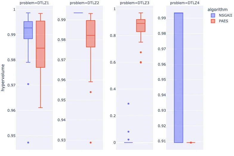
With our data adequately angled, we can produce our visualisation.
fig = px.box(
    df_results,
    facet_col="problem",
    y="hypervolume",
    color="algorithm",
    facet_col_spacing=0.07
)
fig.update_yaxes(matches=None, showticklabels=True)
fig.show()
At a glance, we can see that this particular implementation of NSGA-II has significantly worse performance when compared to PAES on the DTLZ3 problem.
It's important to understand that these complex algorithms have been implemented many times by different engineers and researchers. The description of complex software and its explanation to a human is a difficult task which can easily lead to misinterpretations4. Therefore, it is likely that two implementations of the same algorithm will produce entirely significantly different performance profiles.
Conclusion
In this section we have demonstrated how we can compare two popular multi-objective evolutionary algorithms on a selection of four test problems using the hypervolume indicator to measure their performance. In this case, we simply compared the mean of a sample of executions per problem per algorithm without consideration for statistical significance, however, this it is important to take this into account to ensure that any differences haven't occurred by chance.
Exercise
Create your own experiment, but this time include different algorithms and problems and determine which algorithm performs the best on each problem.
-
Deb, K., Pratap, A., Agarwal, S., & Meyarivan, T. A. M. T. (2002). A fast and elitist multiobjective genetic algorithm: NSGA-II. IEEE transactions on evolutionary computation, 6(2), 182-197. ↩
-
Knowles, J., & Corne, D. (1999, July). The pareto archived evolution strategy: A new baseline algorithm for pareto multiobjective optimisation. In Congress on Evolutionary Computation (CEC99) (Vol. 1, pp. 98-105). ↩
-
Deb, K., Thiele, L., Laumanns, M., & Zitzler, E. (2002, May). Scalable multi-objective optimization test problems. In Proceedings of the 2002 Congress on Evolutionary Computation. CEC'02 (Cat. No. 02TH8600) (Vol. 1, pp. 825-830). IEEE. ↩
-
Rostami, S., Neri, F., & Gyaurski, K. (2020). On algorithmic descriptions and software implementations for multi-objective optimisation: A comparative study. SN Computer Science, 1(5), 1-23. ↩