Population Initialisation

Preamble¶

Introduction¶

Before the main optimisation process (the "generational loop") can begin, we need to complete the initialisation stage of the algorithm. Typically, this involves generating the initial population of solutions by randomly sampling the search-space. We can see in the figure below that this initialisation stage is the first real stage, and it's only executed once. There are many schemes for generating the initial population, and some even include simply loading in a population from an earlier run of an algorithm.

Randomly sampling the search-space¶

When generating an initial population, it's often desirable to have a diverse representation of the search space. This supports better exploitation of problem variables earlier on in the search, without having to rely solely on exploration operators.

We previously defined a solution $x$ as consisting of many problem variables.

$$ x=\langle x_{1},x_{2},\ldots,x_{\mathrm{D}} \rangle \tag{1} $$

We also defined a multi-objective function $f(x)$ as consisting of many objectives.

$$ f(x) =(f_{1}(x),f_{2}(x),\ldots,f_{M}(x))\tag{2} $$

However, we need to have a closer look at how we describe a general multi-objective optimisation problem before we initialise our initial population.

$$ \left.\begin{array}{lll}\tag{3} optimise & f_{m}(x), & m=1,2,\ldots,\mathrm{M};\\ subject\, to & g_{j}(x)\geq0, & j=1,2,\ldots,J;\\ & h_{k}(x)=0, & k=1,2,\ldots,K;\\ & x_{d}^{(L)}\leq x_{d}\leq x_{d}^{(U)} & d=1,2,\ldots,\mathrm{D}; \end{array}\right\} $$

We may already be familiar with some parts of Equation 3, but there are some we haven't covered yet. There are $\mathrm{M}$ objective functions which can be either minimised or maximised. The constraint functions $g_j(x)$ and $h_k(x)$ impose inequality and equality constraints which must be satisfied by a solution $x$ for it to be considered a feasible solution. Another condition which affects the feasibility of a solution $x$ is whether the problem variables fall between (inclusively) the lower $x_{d}^{(L)}$ and upper $x_{d}^{(U)}$ boundaries within the decision space.

The lower $x_{d}^{(L)}$ and upper $x_{d}^{(U)}$ boundaries may not be the same for each problem variable. For example, we can define the following upper and lower boundaries for a problem with 10 problem variables.

In Python, we normally use np.random.rand() to generate random numbers. If we want to generate a population of 20 solutions, each with 10 problem variables ($\mathrm{D} = 10$), we could try something like the following.

This works fine if all of our problem variables are to be within the boundaries 0 and 1 ($x_d \in [0,1]$). However, in this case, we have 10 different upper and lower boundaries, so we can use np.random.uniform() instead.

Let's double-check to make sure our solutions fall within the problem variable boundaries.

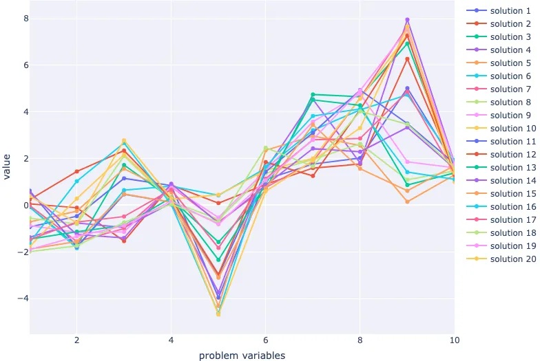
Great! Now all that's left is to visualise our population in the decision space. We'll use a parallel coordinate plot.

To compare one variable to another, we may also want to use a scatterplot matrix.

Conclusion¶

In this section, we had a closer look at multi-objective problems so that we knew how we could complete the initialisation stage in an evolutionary algorithm. We generated a population of solutions within upper and lower boundaries, checked to make sure the problem variables fell between the boundaries, and then visualised them using a scatterplot matrix and parallel coordinate plot. In a simple evolutionary algorithm, we have a population that is ready to enter the generational loop.